Designing database is an integral part of any data application — one that will determine how secure, reliable, and easy to use your entire database application is. To help us design good databases, we have classes of rules we must follow. These classes are called Normal Forms and the process of converting our database into one of these classes is called Normalization.

Normalization

Redundancy is a bad thing most of the time. It takes up extra storage space, it leads to inconsistencies if only one set of redundant data is updated, and it also requires to extra operations to ensure all redundant data is updated at the same time. Database normalization fixes this problem by giving us simple rules to make sure we reduce redundancy in our database. Each class of rule is called a Normal Form and there are 5 normal forms.

What are Normal Forms

Normal Forms are levels of how “good” or reliable our database is. So, your database must be in the first normal form to be at least usable, the third normal form to be good, and the fifth normal form to be really good for most applications.

Example we’ll use throughout the blog:

Suppose we are designing a database for a RPG game where we have users, their levels (beginner, intermediate, advanced), and their inventories. This is a simple database but can help us understand the first few normal forms

The First Normal Form

For a database to be in the first normal form, it must adhere to 3 simple rules:

• You can’t use row order to communicate ranking/order
• No mixing of data types in a single column
• Every table must have a primary key
• No repeating groups (multivalued attributes)

To store the information regarding our users, suppose we use a single table that looks like this:

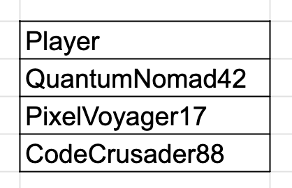
But we also need some sort of ranking for our awards and achievements system. So I propose that we order the users according to their rank. So “QuantumNoma42” has the highest ranking and “CodeCrusader88” has the lowest. If we do that, we’ll be violating the first normal form. To have an actual ranking, we must create another column and store the ranks there

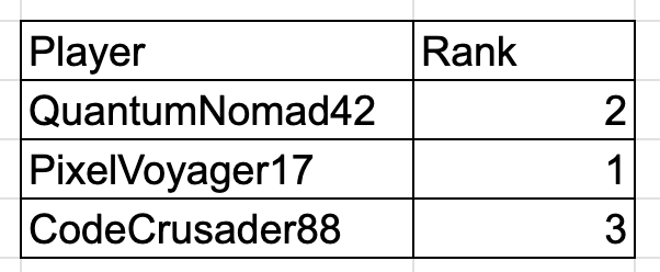
Then in our derived views, we can order the players based on the Rank column.

Secondly, if we mix data types in one of the columns, like if we have strings in our rank:

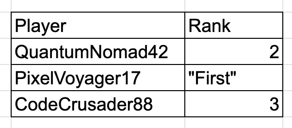
Then we’ll also be violating the first normal form. Most DBMS softwares won’t allow us to do this in the first place. If we say that the “Rank” column is integer, then only integers should be allowed — no mixing of data types.

Lastly, our current database doesn’t stop us from doing this:

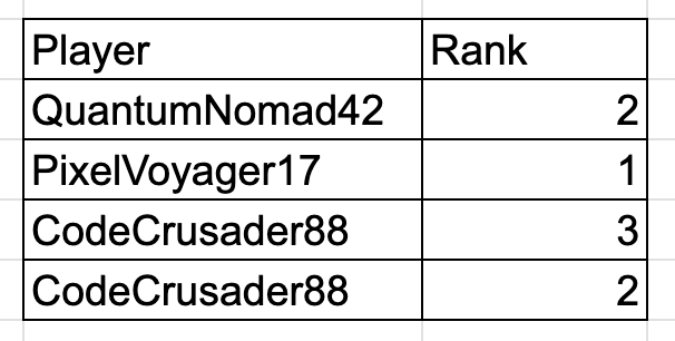
This leads to inconsistency in our data. How can CodeCrusader88 be the second and the third rank at the same time? This also violates the first Normal Principle. To fix this, we need to tell our DBMS software that the Player column is unique — that is, no two rows can have the same Player value. To illustrate this, I’ll underline the Player column:

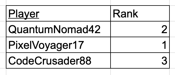
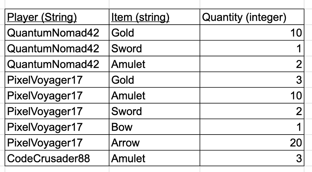
Suppose each player also has an inventory, how may we represent such a system in our database.

Each player has a varying number of items and quantities of each items in their inventories, so a very simple solution would be to store the inventory as a string:

This approach is clearly riddled with problems. What if PixelVoyager17 had 300 different items, our strings would be huge then. And we can’t even query our database properly. What if we need to search for all players with a special amulet? We’ll have to get each player’s inventory string, and use some string searching algorithm like regex. That’s slow and just awkward.

Another way would be to have 10 columns represents the 5 items and the 5 quantities of each item. But that limits our inventory to only 5 items. How could we efficiently store this data.

The inventory column is known as a repeat group (A single cell is storing multiple cells)— This also violates the first normal form. The way to solve this is to have repeating rows, each with just 1 item and its quantity:

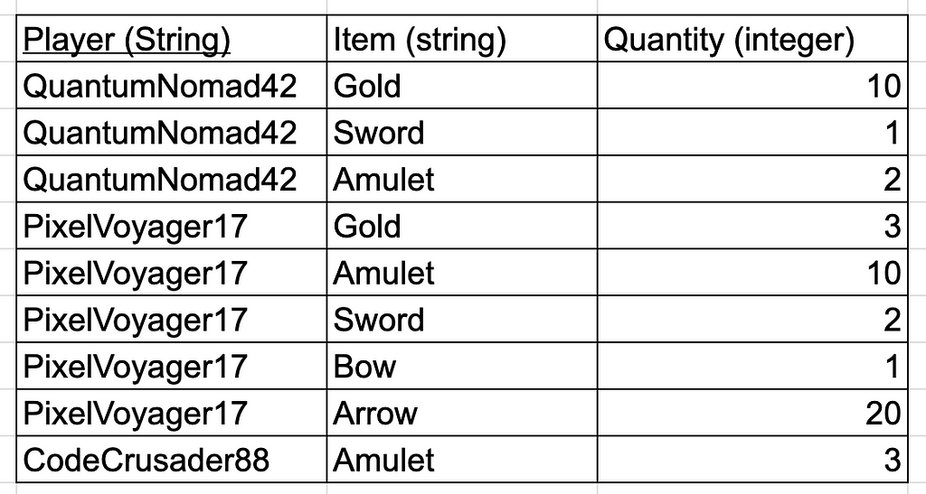
This way, if a player has 300 items, then they’ll just have 300 rows in our table, which is completely fine. “HEY! didn’t you just say that having repeating player names will violate first normal form?” Yes, you’re right, that is why we need to have two primary keys: Player and Item

Having two primary keys basically means that the specific combination of player and item represents the primary key of the table. So, we still have 1 primary key and this time no repeat groups. We can query this database easily to find out the inventory of each player:

SELECT * FROM PLAYER_INVENTORIES WHERE Player='QuantumNomad42'

Or, we could also check which players have a special item

SELECT * FROM PLAYER_INVENTORIES WHERE item='Bow'

Now our database is in first normal form. Just these 4 simple constraints already make our database really nice to work with and reliable.

Second Normal Form

• Each non-key (non-primary) attribute must depend on the entire primary key

Continuing with our inventory table, what if we also want to add the rank of a player and we decide to just willy-nilly add it to the inventory table

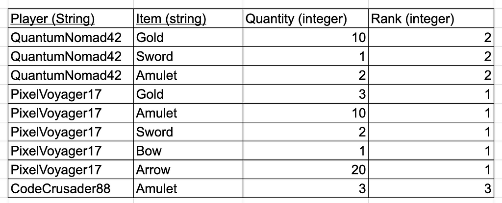
This table passes all the checks for the first normal form, but it has 3 problems:

Deletion Anomaly

Suppose that CodeCrusader88 runs out of arrows, then suddenly that row will be removed from our table. Now we lose all information on that player — their rank, their username, and any other columns we might have had. So this means all players must have something in their inventory to be part of our game? That makes no sense.

Insertion Anomaly

What about someone who just joined? How do we add them in this table? They clearly will have nothing in their inventory, so we simply can’t add them.

Updation Anomaly

Suppose that QuantumNomad42 improved their ranks and now is the first rank. We would have to update all his rows in the table to reflect this. What if we miss a row by mistake? Now we have inconsistent and contradictory data.

To fix these anomalies, we convert our database into the second normal form. The condition for this form is:

• Each non-key (non-primary) attribute must depend on the entire primary key

In our column we have a composite primary key: A key made of the Player and the Item. This condition says that any other column we have in the table must be dependent on both of these primary keys. Clearly the quantity column depends on both of them:

• The same player has different quantities for different items so quantity depends on item (QuantumNomad42 has 10 gold but 1 sword)
• Different players have different quantities of the same item so quantity depends on player (QuantumNomad42 has 1 sword but PixelVoyager17 has 2 swords)

So the quantity column depends on the entire primary key.

The Rank column DOES NOT depend on the entire primary key.

• The Rank column clearly depends on the Player column, since different players have different ranks
• The Rank column doesn’t depend on the item column — since its only concerned with the Player.

So this means that this table violates the Second Normal Form. The easiest way to fix this would be to create another table for the Players and their Ranks

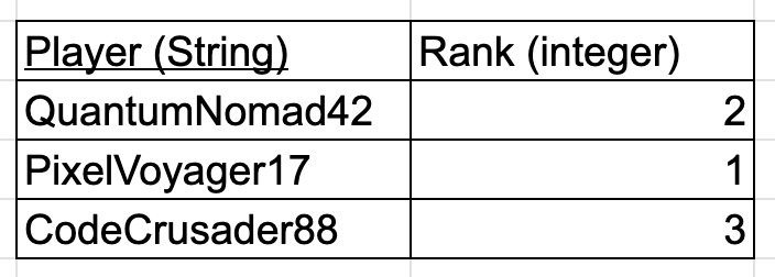
Now we have 2 columns, both of which are in the first and second Normal Forms.

The Third Normal Form

• No non-key attribute must depend on another non-key attribute

Let’s look at the player table once again. Now, we also have a level for each player, ranging from 1 to 10. Level 1 means you’re a noob and level 10 means you’re a pro at the game:

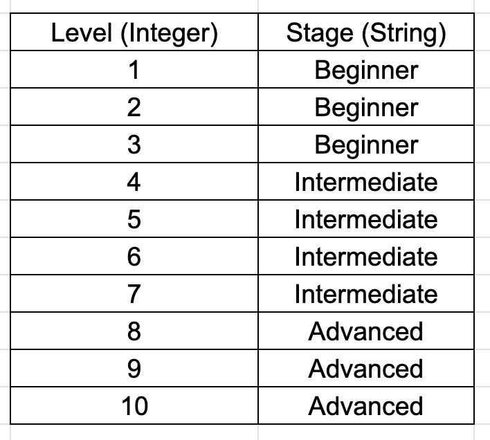
Suppose we have a more subjective column called stage — including a beginner, intermediate, and advanced stage. Suppose anywhere from level 1 to level 3 is beginner, level 4 to level 7 is intermediate, and level 8 to level 10 is advanced:

This table is in the second normal form. But, we have an issue: If the level of CodeCrusader88 increases from 2 to 4, then we must update their stage. If we don’t then we have a logical contradiction in our database. And due to errors or mistakes, that is a very likely scenario. And what if their level increase from 4 to 5, and they’ve surpassed QuantumNomad42. In this case we need to change both the Stage column and the Rank column. Our database modification queries are becoming more complex and can be easily mistaken. This is happening because we’re violating the Third Normal Form.

Look at this:

• The Level column solely depends on the Player column
• The Stage Column depends on the Level column and then the Player column
• The Rank Column depends an ordering based off the level column.

Essentially, the Level column depends on the primary key of the table but the Stage and Rank columns depend on the level column which is a non-primary column of the table. This is not allowed in the Third Normal Form.

In the Third Normal Form, all non-primary/non-key columns cannot depend on other non-primary/non-key columns. To fix this, we must do two things:

We remove the Stage column and make a new table out of each level and stage. In this table we have all the levels from 1 to 10 and the related Stages

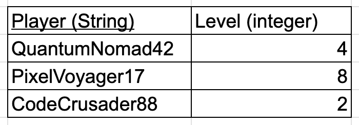
We remove the Rank column and depend on an external “view” to order the players based on level and rank them.

SELECT * FROM players ORDER BY Level

The Fourth Normal Form

• Multivalued dependencies must only be dependent on the key

Suppose in the game, we have a item shop with 3 items: Armor, Swords, and bows. We have each item made from different materials and different levels:

Armor:

• Materials: Iron, Gold, Obsidian
• Levels: 1, 2, 3

Sword:

• Material: Glass, Steel, Diamond
• Levels: 1, 2

Bows:

• Materials: Wood, Steel
• Level: 1, 2, 3

How would you model this information in a database? A first thought would be something like this

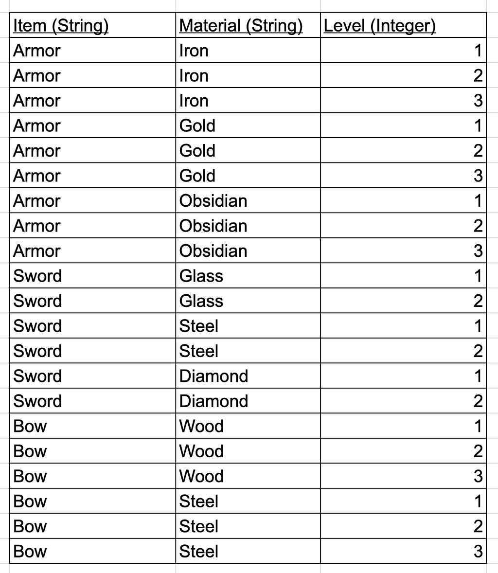
We have every possible combination listed out. But you can already see a lot of problems.

Armors had 3 materials and 3 levels, so I had to make 9 rows. What if armor had 20 different levels? I would have to make 60 rows. Also what if I need to add another material to Bow? I would have to create 3 new rows for each level. What if after that, I need to add another level to Bow? I would have to create 3 new rows for each of the materials. All this updating can definitely be error prone and is not a good practice. This is because this table violates the Fourth Normal Form:

• Multivalued dependencies must only be dependent on the key

Both the Material and the Level columns are multi-valued. The Fourth Normal Form says that these columns must only be dependent on the key (primary-key). But, in our column our primary key is actually all 3 columns. So, we cannot say that any of these columns are dependent on the key (they literally make up the key so they can’t be dependent on it).

To fix this, we break our big table into 2 smaller tables:

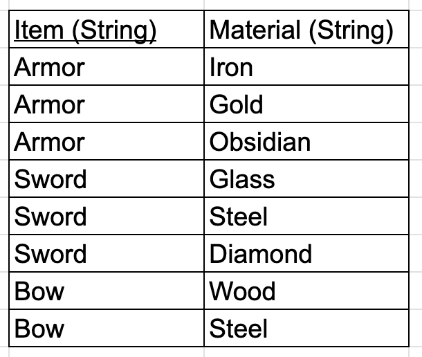
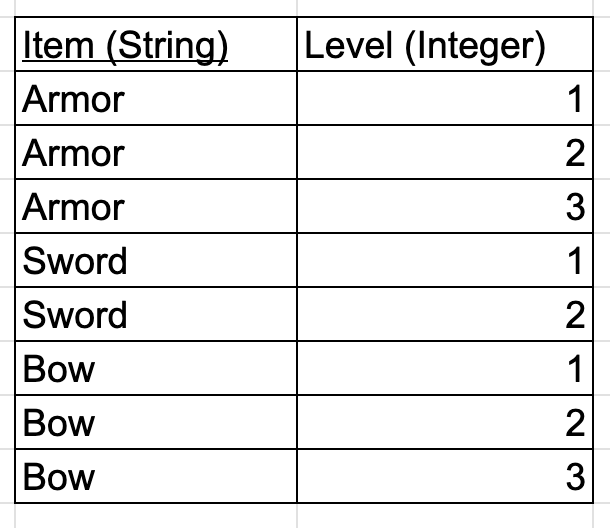
Now, our tables are in the Fourth Normal Form as well.

The Fifth Normal Form

• If the table can be thought of as join between multiple tables, it isn’t in the fifth normal form

Suppose now we want to track not only players and items, but also which quests they have completed and what items they used for those quests. We may initially design a table like this:

This table shows which items players used for specific quests. However, this table might have unnecessary redundancy if the relationships between players, items, and quests can be separated into smaller tables.

The key here is to avoid storing repetitive data that can be represented using multiple smaller, normalized tables.

We can decompose this table into three smaller tables like this:

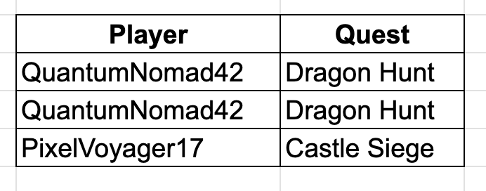
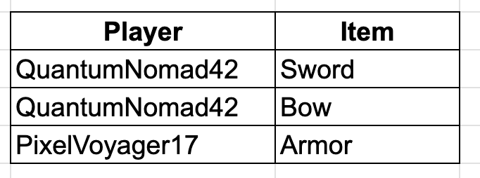
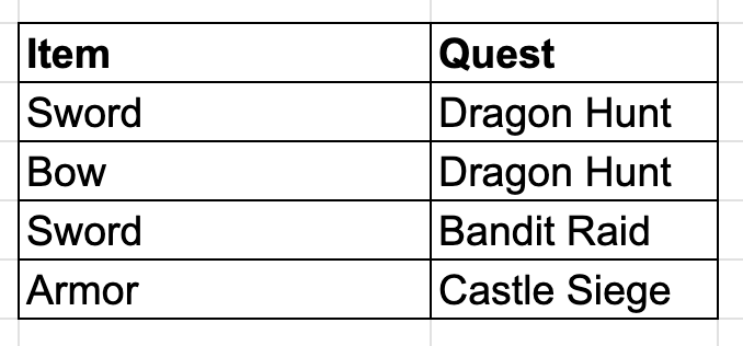
This way, we have the same information but stored in smaller, easier to handle and store tables.

What’s the difference between The Fourth and Fifth Normal Form:

The Fourth Normal Form address redundancies due to multivalued columns, while the Fifth normal Form address redundancies due to a “joined” table which can be decomposed into smaller ones.

Conclusion

Database normalization is a crucial step in ensuring that a database is well-structured, efficient, and free from redundancy and update anomalies. As we progress through the normal forms, each level builds on the previous one, addressing more complex forms of data dependencies and relationships.

• 1NF eliminates repeating groups and ensures “atomicity”.
• 2NF ensures that every non-key attribute depends on the entire primary key.
• 3NF removes transitive dependencies between non-key attributes.
• 4NF deals with multivalued dependencies to avoid redundancy.
• 5NF ensures the elimination of redundancy by decomposing tables where join dependencies exist.

Ultimately, by reaching 5NF, your database will be optimized, scalable, and maintainable, capable of handling complex relationships with minimal redundancy.